Breast Cancer Prediction Using Machine Learning
Breast cancer, one of the most prevalent forms of cancer, affects millions of lives worldwide. Early detection significantly enhances the chances of successful treatment. In this blog post, we will explore how cutting-edge machine learning techniques can empower healthcare professionals by predicting breast cancer with high accuracy. We’ll dive into the world of data, algorithms, and empowerment through technology.
What is Breast Cancer
Cancer is a broad term for a class of diseases characterized by abnormal cells that grow and invade healthy cells in the body. Breast cancer starts in the cells of the breast as a group of cancer cells that can then invade surrounding tissues or spread (metastasize) to other areas of the body. Breast cancer is a disease in which malignant (cancer) cells form in the tissues of the breast.
What Causes Breast Cancer
Cancer begins in the cells which are the basic building blocks that make up tissue. Tissue is found in the breast and other parts of the body. Sometimes, the process of cell growth goes wrong and new cells form when the body doesn’t need them and old or damaged cells do not die as they should. When this occurs, a build-up of cells often forms a mass of tissue called a lump, growth, or tumor.
Breast cancer occurs when malignant tumors develop in the breast. These cells can spread by breaking away from the original tumor and entering blood vessels or lymph vessels, branching into tissues throughout the body. When cancer cells travel to other parts of the body and begin damaging other tissues and organs, the process is called metastasis.
What Is A Tumor
A tumor is a mass of abnormal tissue. There are two types of breast cancer tumors: those that are non-cancerous, or ‘benign’, and those that are cancerous, which are ‘malignant’.
Benign Tumors
When a tumor is diagnosed as benign, doctors will usually leave it alone rather than remove it. Even though these tumors are not generally aggressive toward surrounding tissue, occasionally they may continue to grow, pressing on other tissue and causing pain or other problems. In these situations, the tumor is removed, allowing pain or complications to subside.
Malignant Tumors
Malignant tumors are cancerous and may be aggressive because they invade and damage surrounding tissue. When a tumor is suspected to be malignant, the doctor will perform a biopsy to determine the severity or aggressiveness of the tumor.
In this study, advanced machine learning methods will be utilized to build and test the performance of a selected algorithm for breast cancer diagnosis.
1. Understanding the Dataset
Our journey begins with a dataset – a collection of valuable information waiting to reveal patterns. The Breast Cancer Wisconsin (Diagnostic) dataset provides a rich set of features derived from cell nuclei characteristics. Each feature is a potential clue in our quest for early cancer detection.
The Breast Cancer Wisconsin (Diagnostic) dataset, often referred to as the “Breast Cancer dataset” or “WBCD dataset,” is a widely used dataset in machine learning for classification tasks. It was created by Dr. William H. Wolberg, W. Nick Street, and Olvi L. Mangasarian from the University of Wisconsin Hospitals, Madison, Wisconsin, USA. The dataset is publicly available and can be accessed through the UCI Machine Learning Repository.
The dataset contains features computed from a digitized image of a fine needle aspirate (FNA) of a breast mass. These features describe the characteristics of the cell nuclei present in the image. The task associated with this dataset is to classify the breast mass as benign (B) or malignant (M) based on these features. Here are the details of the dataset:
- Number of Instances: 569
- Number of Features: 30 numeric, real-valued features are computed from cell nuclei characteristics
- Attribute Information:
-
- ID Number: Unique identification number
- Diagnosis (M or B): Malignant (cancerous) or Benign (non-cancerous)
- (3-30) Ten real-valued features are computed for each cell nucleus:
- Radius (mean of distances from the center to points on the perimeter)
- Texture (standard deviation of gray-scale values)
- Perimeter
- Area
- Smoothness (local variation in radius lengths)
- Compactness (perimeter^2 / area – 1.0)
- Concavity (severity of concave portions of the contour)
- Concave points (number of concave portions of the contour)
- Symmetry
- Fractal dimension (“coastline approximation” – 1)
For each of these ten features, the mean, standard error, and “worst” or largest (mean of the three largest values) values are computed, resulting in 30 features.
-
2. Data Exploration
To understand the dataset we need to explore the dataset first. Here are the top 5 records of the dataset:
| id | diagnosis | radius_mean | … | symmetry_worst | fractal_dimension_worst | Unnamed: 32 | |
|---|---|---|---|---|---|---|---|
| 0 | 842302 | M | 17.99 | … | 0.4601 | 0.11890 | NaN |
| 1 | 842517 | M | 20.57 | … | 0.2750 | 0.08902 | NaN |
| 2 | 84300903 | M | 19.69 | … | 0.3613 | 0.08758 | NaN |
| 3 | 84348301 | M | 11.42 | … | 0.6638 | 0.17300 | NaN |
| 4 | 84358402 | M | 20.29 | … | 0.2364 | 0.07678 | NaN |
Here are some broad-level statistics of the dataset:
| count | mean | std | … | 50% | 75% | max | |
|---|---|---|---|---|---|---|---|
| id | 569.0 | 3.037183e+07 | 1.250206e+08 | … | 906024.000000 | 8.813129e+06 | 9.113205e+08 |
| radius_mean | 569.0 | 1.412729e+01 | 3.524049e+00 | … | 13.370000 | 1.578000e+01 | 2.811000e+01 |
| texture_mean | 569.0 | 1.928965e+01 | 4.301036e+00 | … | 18.840000 | 2.180000e+01 | 3.928000e+01 |
| perimeter_mean | 569.0 | 9.196903e+01 | 2.429898e+01 | … | 86.240000 | 1.041000e+02 | 1.885000e+02 |
| area_mean | 569.0 | 6.548891e+02 | 3.519141e+02 | … | 551.100000 | 7.827000e+02 | 2.501000e+03 |
| smoothness_mean | 569.0 | 9.636028e-02 | 1.406413e-02 | … | 0.095870 | 1.053000e-01 | 1.634000e-01 |
| compactness_mean | 569.0 | 1.043410e-01 | 5.281276e-02 | … | 0.092630 | 1.304000e-01 | 3.454000e-01 |
| concavity_mean | 569.0 | 8.879932e-02 | 7.971981e-02 | … | 0.061540 | 1.307000e-01 | 4.268000e-01 |
| concave points_mean | 569.0 | 4.891915e-02 | 3.880284e-02 | … | 0.033500 | 7.400000e-02 | 2.012000e-01 |
| symmetry_mean | 569.0 | 1.811619e-01 | 2.741428e-02 | … | 0.179200 | 1.957000e-01 | 3.040000e-01 |
| fractal_dimension_mean | 569.0 | 6.279761e-02 | 7.060363e-03 | … | 0.061540 | 6.612000e-02 | 9.744000e-02 |
| radius_se | 569.0 | 4.051721e-01 | 2.773127e-01 | … | 0.324200 | 4.789000e-01 | 2.873000e+00 |
| texture_se | 569.0 | 1.216853e+00 | 5.516484e-01 | … | 1.108000 | 1.474000e+00 | 4.885000e+00 |
| perimeter_se | 569.0 | 2.866059e+00 | 2.021855e+00 | … | 2.287000 | 3.357000e+00 | 2.198000e+01 |
| area_se | 569.0 | 4.033708e+01 | 4.549101e+01 | … | 24.530000 | 4.519000e+01 | 5.422000e+02 |
| smoothness_se | 569.0 | 7.040979e-03 | 3.002518e-03 | … | 0.006380 | 8.146000e-03 | 3.113000e-02 |
| compactness_se | 569.0 | 2.547814e-02 | 1.790818e-02 | … | 0.020450 | 3.245000e-02 | 1.354000e-01 |
| concavity_se | 569.0 | 3.189372e-02 | 3.018606e-02 | … | 0.025890 | 4.205000e-02 | 3.960000e-01 |
| concave points_se | 569.0 | 1.179614e-02 | 6.170285e-03 | … | 0.010930 | 1.471000e-02 | 5.279000e-02 |
| symmetry_se | 569.0 | 2.054230e-02 | 8.266372e-03 | … | 0.018730 | 2.348000e-02 | 7.895000e-02 |
| fractal_dimension_se | 569.0 | 3.794904e-03 | 2.646071e-03 | … | 0.003187 | 4.558000e-03 | 2.984000e-02 |
| radius_worst | 569.0 | 1.626919e+01 | 4.833242e+00 | … | 14.970000 | 1.879000e+01 | 3.604000e+01 |
| texture_worst | 569.0 | 2.567722e+01 | 6.146258e+00 | … | 25.410000 | 2.972000e+01 | 4.954000e+01 |
| perimeter_worst | 569.0 | 1.072612e+02 | 3.360254e+01 | … | 97.660000 | 1.254000e+02 | 2.512000e+02 |
| area_worst | 569.0 | 8.805831e+02 | 5.693570e+02 | … | 686.500000 | 1.084000e+03 | 4.254000e+03 |
| smoothness_worst | 569.0 | 1.323686e-01 | 2.283243e-02 | … | 0.131300 | 1.460000e-01 | 2.226000e-01 |
| compactness_worst | 569.0 | 2.542650e-01 | 1.573365e-01 | … | 0.211900 | 3.391000e-01 | 1.058000e+00 |
| concavity_worst | 569.0 | 2.721885e-01 | 2.086243e-01 | … | 0.226700 | 3.829000e-01 | 1.252000e+00 |
| concave points_worst | 569.0 | 1.146062e-01 | 6.573234e-02 | … | 0.099930 | 1.614000e-01 | 2.910000e-01 |
| symmetry_worst | 569.0 | 2.900756e-01 | 6.186747e-02 | … | 0.282200 | 3.179000e-01 | 6.638000e-01 |
| fractal_dimension_worst | 569.0 | 8.394582e-02 | 1.806127e-02 | … | 0.080040 | 9.208000e-02 | 2.075000e-01 |
| Unnamed: 32 | 0.0 | NaN | NaN | … | NaN | NaN | NaN |
Here are the datatypes of the dataset:
id                           int64
diagnosis                   object
radius_mean                float64
texture_mean               float64
perimeter_mean             float64
area_mean                  float64
smoothness_mean            float64
compactness_mean           float64
concavity_mean             float64
concave points_mean        float64
symmetry_mean              float64
fractal_dimension_mean     float64
radius_se                  float64
texture_se                 float64
perimeter_se               float64
area_se                    float64
smoothness_se              float64
compactness_se             float64
concavity_se               float64
concave points_se          float64
symmetry_se                float64
fractal_dimension_se       float64
radius_worst               float64
texture_worst              float64
perimeter_worst            float64
area_worst                 float64
smoothness_worst           float64
compactness_worst          float64
concavity_worst            float64
concave points_worst       float64
symmetry_worst             float64
fractal_dimension_worst    float64
Unnamed: 32                float64
dtype: object
We are going to do the following things from the above statistics:
1. Delete the column “Unnamed: 32”
2. Map 1 for “M” and 0 for “B” in the diagnosis column
3. Correlation Among Fields and Taking Actions
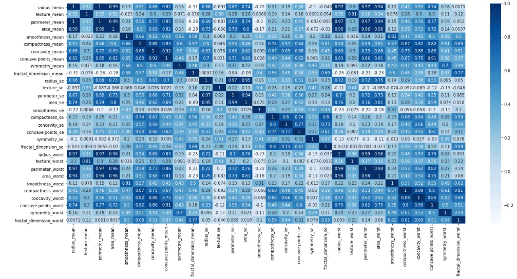
Now, let’s see the correlation among fields. Here is the result:

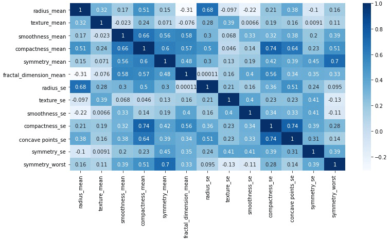
While we look into the above matrix we can find out the fields to be removed. We see ‘area_mean’, ‘area_se’, ‘area_worst’, ‘compactness_worst’, ‘concave points_mean’, ‘concave points_worst’, ‘concavity_mean’, ‘concavity_se’, ‘concavity_worst’, ‘fractal_dimension_se’, ‘fractal_dimension_worst’, ‘perimeter_mean’, ‘perimeter_se’, ‘perimeter_worst’, ‘radius_worst’, ‘smoothness_worst’, ‘texture_worst’ are very much correlated to each other. So, after removing them we will see a matrix as below:

4. Data Preprocessing
Ensuring data quality is paramount. We preprocess the data by standardizing features. Now, it’s time to standardize all numerical values. To do that, we will use the StandardScaler() function as below.
# Data Preprocessing
from sklearn.model_selection import train_test_split
from sklearn.preprocessing import StandardScaler

scaler = StandardScaler()
X_scaled = scaler.fit_transform(X)
After transforming the dataset it will look like as below:
[ 1.09706398e+00, -2.07333501e+00,  1.56846633e+00, 3.28351467e+00,  2.21751501e+00,  2.25574689e+00, 2.48973393e+00, -5.65265059e-01, -2.14001647e-01, 1.31686157e+00,  6.60819941e-01,  1.14875667e+00, 2.75062224e+00],
[ 1.82982061e+00, -3.53632408e-01, -8.26962447e-01,  -4.87071673e-01,  1.39236330e-03, -8.68652457e-01, 4.99254601e-01, -8.76243603e-01, -6.05350847e-01, -6.92926270e-01,  2.60162067e-01, -8.05450380e-01, -2.43889668e-01],
[ 1.57988811e+00,  4.56186952e-01,  9.42210440e-01, 1.05292554e+00,  9.39684817e-01, -3.98007910e-01, 1.22867595e+00, -7.80083377e-01, -2.97005012e-01, 8.14973504e-01,  1.42482747e+00,  2.37035535e-01, 1.15225500e+00],
[-7.68909287e-01,  2.53732112e-01,  3.28355348e+00, 3.40290899e+00,  2.86738293e+00,  4.91091929e+00, 3.26373441e-01, -1.10409044e-01,  6.89701660e-01, 2.74428041e+00,  1.11500701e+00,  4.73268037e+00, 6.04604135e+00],
[ 1.75029663e+00, -1.15181643e+00,  2.80371830e-01, 5.39340452e-01, -9.56046689e-03, -5.62449981e-01, 1.27054278e+00, -7.90243702e-01,  1.48306716e+00, -4.85198799e-02,  1.14420474e+00, -3.61092272e-01, -8.68352984e-01]
5. Training Models
Before training the model we split the dataset into Training (80%) and Testing Datasets (20%) by stratified sampling method. The heart of our solution lies in a machine learning model. Now we are ready to train our machine using different machine learning algorithms. There are many algorithms in Python to train our machine. We have used 9 most popular algorithms to train our machine and have built 9 different ones to create our breast cancer prediction models. Overall, the process will take some time to train our machine with those selected algorithms. It will depend mainly on the capacity of the processor & random access memory of our machine.
6. Model Evaluation and Empowerment
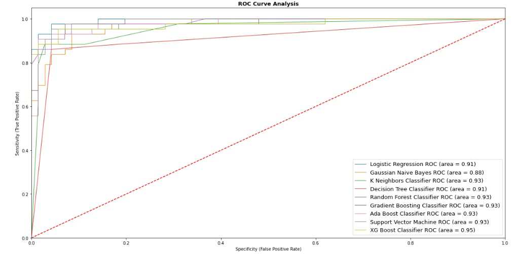
After completion of the model building process, we have to see the performance of different models. One algorithm can not be the best for all kinds of datasets. Our models are now ready to face the ultimate test – real-world data. By evaluating its performance, we gauge its accuracy and effectiveness. Let’s see the performance of these 8 models using 9 Machine Learning algorithms:

| Model_Name | Jaccard_Score | Accuracy_Score | F1_Score | LogLoss | |
|---|---|---|---|---|---|
| 8 | XGBoost Classifier | 0.872340 | 0.947368 | 0.947591 | 1.897034 |
| 5 | Gradient Boosting Classifier | 0.847826 | 0.938596 | 0.938450 | 2.213207 |
| 6 | Ada Boost Classifier | 0.847826 | 0.938596 | 0.938450 | 2.213207 |
| 7 | Support Vector Machine | 0.847826 | 0.938596 | 0.938450 | 2.213207 |
| 2 | K Neighbors Classifier | 0.844444 | 0.938596 | 0.938122 | 2.213207 |
| 4 | Random Forest Classifier | 0.829787 | 0.929825 | 0.929825 | 2.529379 |
| 0 | Logistic Regression | 0.813953 | 0.929825 | 0.928097 | 2.529379 |
| 3 | Decision Tree Classifier | 0.804348 | 0.921053 | 0.920443 | 2.845552 |
| 1 | Gaussian Naive Bayes | 0.750000 | 0.894737 | 0.894215 | 3.794069 |
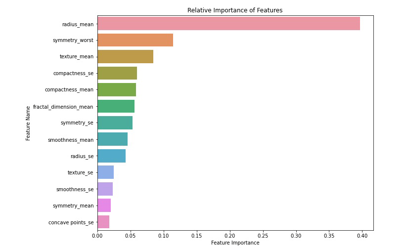
According to the above performance graph and result data, it is clear that the “XGBoost Classifier” is showing the highest performance among all models. So, we have selected “XGBoost Classifier” as our final algorithm with an accuracy score of 94.74%. Now let’s see the relative importance of the features to identify breast cancer is as below:

| Feature_Name | Relative_Importance | |
|---|---|---|
| 0 | radius_mean | 0.396653 |
| 12 | symmetry_worst | 0.114696 |
| 1 | texture_mean | 0.084287 |
| 9 | compactness_se | 0.060002 |
| 3 | compactness_mean | 0.058612 |
| 5 | fractal_dimension_mean | 0.056233 |
| 11 | symmetry_se | 0.053392 |
| 2 | smoothness_mean | 0.045545 |
| 6 | radius_se | 0.042849 |
| 7 | texture_se | 0.025224 |
| 8 | smoothness_se | 0.023318 |
| 4 | symmetry_mean | 0.020734 |
| 10 | concave points_se | 0.018455 |
So, we see that the most important feature to identify breast cancer is radius_mean followed by radius_se, compactness_mean… Through the power of machine learning, we’ve created a tool capable of aiding medical professionals in their battle against breast cancer. With high accuracy and the ability to process vast amounts of data, machine learning stands as a beacon of hope, enabling earlier detection and, ultimately, saving lives.
Conclusion
Breast cancer detection using machine learning in Python is a powerful application that showcases the potential of AI in healthcare. By following these steps and understanding the underlying concepts, you can create a robust breast cancer detection system using machine learning. Remember, continuous learning and experimentation are key to mastering these techniques and making a real impact in the field of healthcare. In this blog post, we’ve embarked on a journey from data to empowerment. Through machine learning, we’ve transformed raw information into a predictive model, empowering healthcare professionals with a potent tool against breast cancer. As technology advances, so does our ability to make a difference. Let us continue harnessing the power of machine learning to shape a healthier, more hopeful future for all. If you want to get updated, you can subscribe to our Facebook page http://www.facebook.com/LearningBigDataAnalytics.

