Titanic Survivors Prediction Using Machine Learning
Titanic, the famous passenger liner that sank on her maiden voyage on the 15th April 1912 following her collision with an iceberg, killing 1,514 out of 2,224 passengers and crew. One of the reasons that the shipwreck led to such loss of life was that there were not enough lifeboats for the passengers and crew. Although there was some element of luck involved in surviving the sinking, some groups of people were more likely to survive than others.
Many data scientists started their first machine learning practice by this datasets. These datasets are very much simple, easy to understand and there are many interesting factors which you can think other way also.
In this article we will show you a step by step process of Titanic survivors prediction using Machine Learning.
1. Understanding The Datasets
‘data.frame’: 1309 obs. of 13 variables:
$ PassengerId: int 1 2 3 4 5 6 7 8 9 10 …
$ Survived : int 0 1 1 1 0 0 0 0 1 1 …
$ Pclass : int 3 1 3 1 3 3 1 3 3 2 …
$ Name : chr “Braund, Mr. Owen Harris” “Cumings, Mrs. John Bradley (Florence Briggs Thayer)” “Heikkinen, Miss. Laina” “Futrelle, Mrs. Jacques Heath (Lily May Peel)” …
$ Sex : chr “male” “female” “female” “female” …
$ Age : num 22 38 26 35 35 NA 54 2 27 14 …
$ SibSp : int 1 1 0 1 0 0 0 3 0 1 …
$ Parch : int 0 0 0 0 0 0 0 1 2 0 …
$ Ticket : chr “A/5 21171” “PC 17599” “STON/O2. 3101282” “113803” …
$ Fare : num 7.25 71.28 7.92 53.1 8.05 …
$ Cabin : chr “” “C85” “” “C123” …
$ Embarked : chr “S” “C” “S” “S” …
$ Cat : chr “Train” “Train” “Train” “Train” …
Let’s see the meaning of the different fields of the titanic dataset:
Passenger ID : Unique number of each passenger
Survived : A binary indicator of survival (1 = survived, 0 = died)
PClass : A proxy for socio-economic status (1 = upper, 3 = lower)
Name : Passenger’s Name. For wedded women, her husband’s name appears first and her maiden name appears in parentheses
Sex : Passenger’s Gender
Age : Age of passenger (Passengers under the age of 1 year have fractional ages and rest of ages are rounded)
SibSp : A count of the passenger’s siblings or spouses aboard
Parch : A count of the passenger’s parents or siblings aboard
Ticket : Ticket number of the passenger
Fare : The price for the ticket (presumably in pounds, shillings, and pennies)
Cabin : Cabin number occupied by the passenger
Embarked : The port from where the passenger boarded the ship
Cat : Derived column to identify whether the dataset was a part of the training or testing
Let’s see the dataset in more details way with one of my own developed functions:
| variable_name | variable_type | record_count | unique_count | empty_count | null_count | missing_count | |
| 1 | PassengerId | numeric | 1309 | 1309 | 0 | 0 | 0 |
| 2 | Survived | numeric | 1309 | 2 | 0 | 0 | 0 |
| 3 | Pclass | numeric | 1309 | 3 | 0 | 0 | 0 |
| 4 | Name | character | 1309 | 1307 | 0 | 0 | 0 |
| 5 | Sex | character | 1309 | 2 | 0 | 0 | 0 |
| 6 | Age | numeric | 1309 | 99 | 0 | 263 | 263 |
| 7 | SibSp | numeric | 1309 | 7 | 0 | 0 | 0 |
| 8 | Parch | numeric | 1309 | 8 | 0 | 0 | 0 |
| 9 | Ticket | character | 1309 | 929 | 0 | 0 | 0 |
| 10 | Fare | numeric | 1309 | 282 | 0 | 1 | 1 |
| 11 | Cabin | character | 1309 | 187 | 1014 | 0 | 1014 |
| 12 | Embarked | character | 1309 | 4 | 2 | 0 | 2 |
| 13 | Cat | character | 1309 | 2 | 0 | 0 | 0 |
In the above data we see that 1 passenger has missing Fare related data, 2 passengers have missing Embarked related data, 263 passengers have missing Age related data and 1,014 passengers have missing Cabin related data.
2. Feature Engineering
A feature is an attribute or property of an independent units of a specific dataset. Any attribute could be a feature, as long as it is useful to the model. Feature engineering is the process to extract features from source data via data processing or data mining techniques. These features can be used to improve the performance of machine learning algorithms.
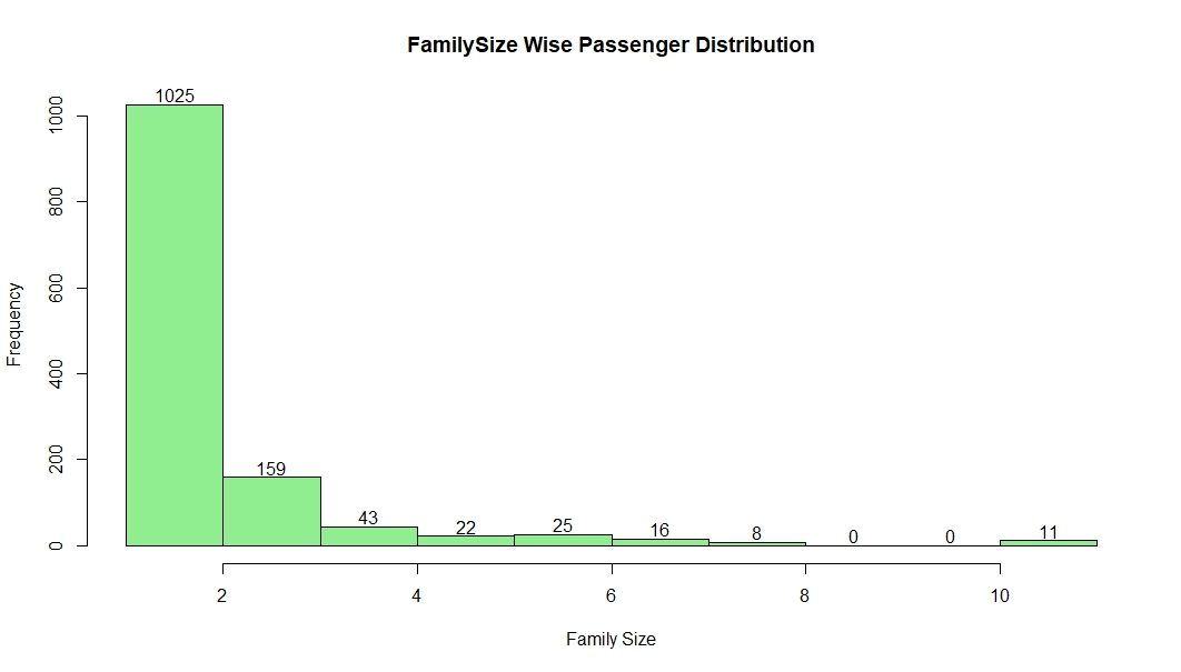
2.1 FamilySize
Since SibSp, Parch are part of family, it would make sense to derive a new variable FamilySize by SibSp & Parch as FamilySize=SibSp+Parch+1. Now, let’s visualize the distribution of new variable FamilySize.
2.2 GroupSize
Since one passenger many have one ticket or multiple passengers may have one ticket. Let’s transpose passengers as group and by these size of the group let’s create a new variable GroupSize. Now, let’s visualize distribution of this new variable GroupSize.

2.3 Title Category
We can analyze the passenger category by his/her name. In Every name there is a title portion. Let’s create a new derived variable Title from name value. Here is the titles of overall passengers:
“Mr” “Mrs” “Miss” “Master” “Don” “Rev”
“Dr” “Mme” “Ms” “Major” “Lady” “Sir”
“Mlle” “Col” “Capt” “the Countess” “Jonkheer” “Dona”
Let’s clap “Dona”, “the Countess”, “Mme” into “Lady” and “Don”, “Jonkheer” into “Sir”.
3. Data Imputation
Data imputation is the process of replacing missing data with substituted values. It is very much important steps in the Machine Learning steps. There are many ways to do this kind of job. Here we will apply some of them.
3.1 Missing Fare
We see that only one record has missing fare value. You can go with different strategy to impute this missing value. Since it is only one value I am preferring to impute with median value. Let’s see the missing record with some related fields.
| PassengerId | PClass | Age | Embarked | CabinCategory | Fare |
| 1044 | 3 | 60.5 | S | N | NA |
Let’s consider PClass, Embarked & CabinCategory to determine the missing Fare. We can look into the median Fare of the passengers of the this category. If we look into the graph we see the median fare of the category is $8.05.
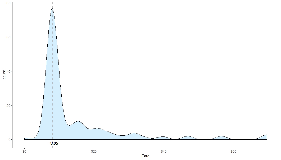
So, I would like the update the missing fare with 8.05.
3.2 Missing Embarked
We see that there are two missing records in this case. We can go with different strategy to impute this missing value. Since it is only two missing values I am preferring to impute with median value of the specific segment. Let’s see the missing record with some related fields.
| PassengerId | PClass | Age | CabinCategory | Fare | Embarked |
| 62 | 1 | 38 | B | 80 | NA |
| 830 | 1 | 62 | B | 80 | NA |
Let’s consider PClass, Fare & CabinCategory to determine the missing Embarked value. We can see which Embarked value has nearest median fare value of 80 with PClass value of “1”.
| Embarked | PClass | CabinCategory | MedianFare | Count | |
| 1 | 1 | B | 80 | 2 | |
| 2 | C | 1 | B | 91.1 | 32 |
| 3 | S | 1 | B | 82.3 | 31 |
According to the above table we see that missing Embarked value is very much similar to the 3rd record since it has Median Fare value is 82.3 which is the nearest value of 80. So, we can update missing Embarked value with “S”.
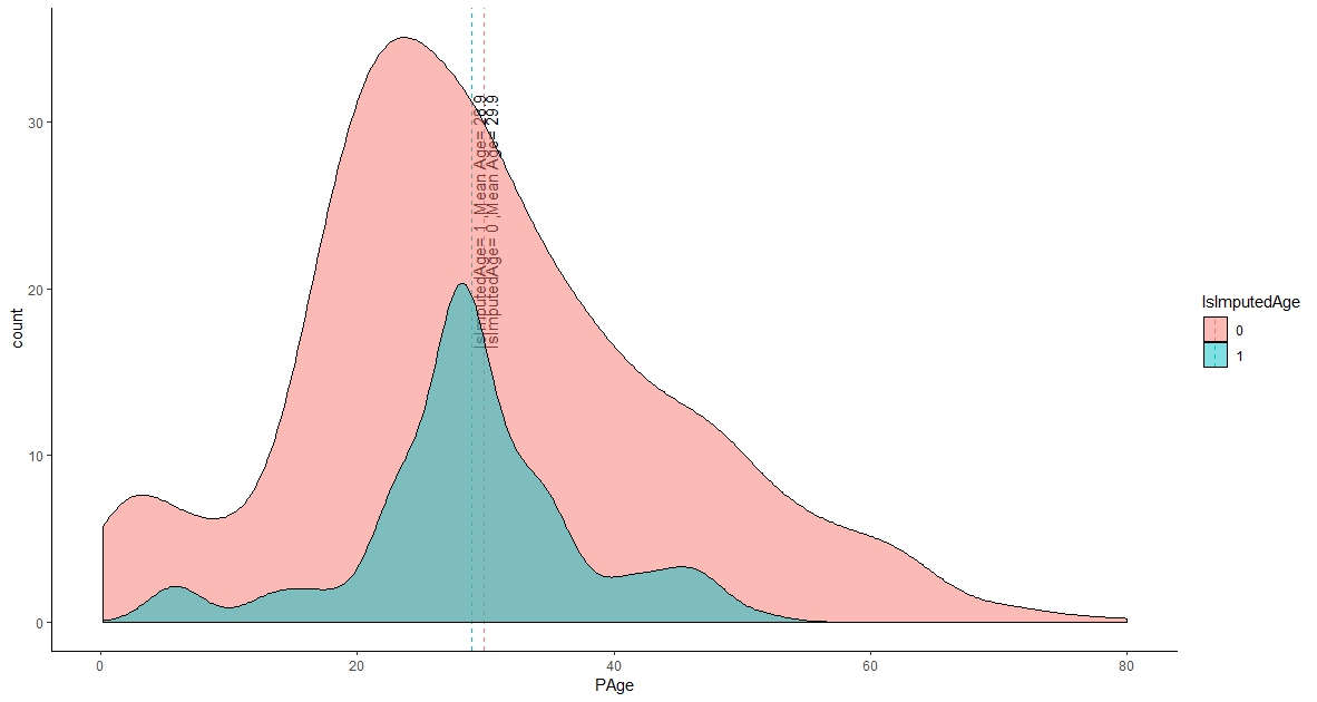
3.3 Missing Age
If we look into the above data summary of section 1, we would see there are 263 passengers who have missing age related value. According to the total record it is huge in numbers. We can replace null values by available median age. But if it is one or two value we can do it by above data exploration process. Since, the number is huge we it will be very much hard for us to do it. On the other note we can say it will not be wise to replace the value with a single value (i.e median, mean or mode values) or do replacement by manually by comparing with other variable rather than regression method. So, In this case we have decided to select regression method using one of the favorite algorithm. After building up the model we have found relative importance of the used variable for predicting missing age as below:

We have replaced our missing age data by model predicted data. Let’s put the existing age related data and imputed age related data into a graph to see the imputed value comparing to existing value. If we look into the below graph, it seems imputed age distribution is very much similar to the existing age. Hope it would give us a good accuracy to our next upcoming model to identify survivors.
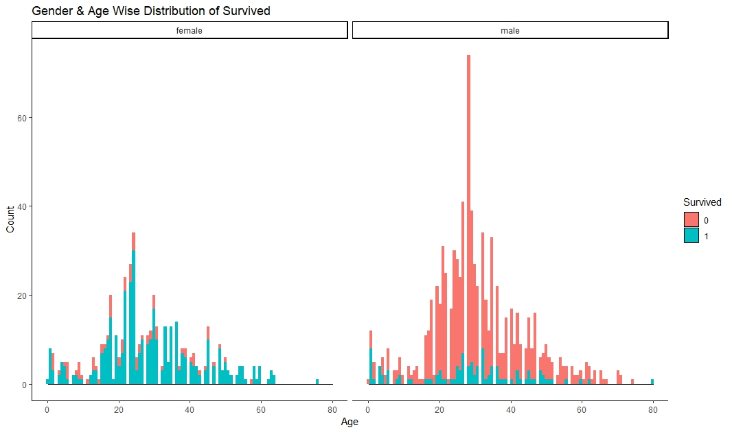
4. Visualize the Data
It seems that female are survived more than male and lower aged are more survived.
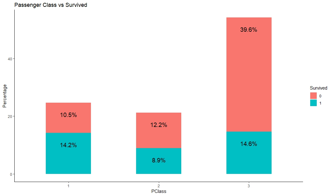
Below graph shows that higher class people are more survived than lower class people.
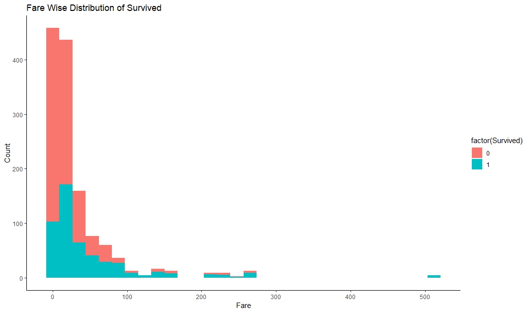
Below graph shows that passenger with higher fare survived more than lower ticket fare.
5. Training Models
Now we are ready to train our machine using different machine learning algorithms. There are many algorithms in R to train our machine. We have used 15 most popular algorithms to train our machine and have built 15 different models. Overall process will take a good amount of time to train our machine with those selected algorithms. It will depends mainly on the capacity of processor & random access memory of our machine.
6. Selecting The Best Model
After completion of the model building process, we have to see the performance of different models. One algorithm can not be the best for all kinds of datasets. It’s time to measure the performance of different models. Let’s see the performance of these 15 models using 15 Machine Learning algorithms:
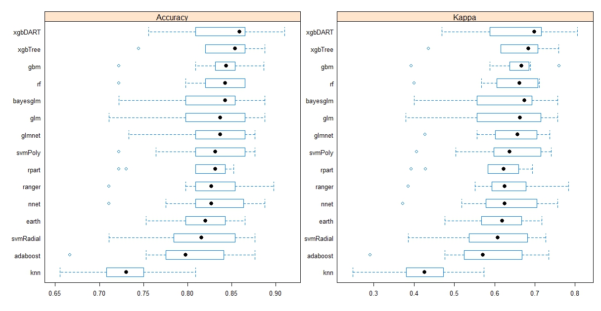
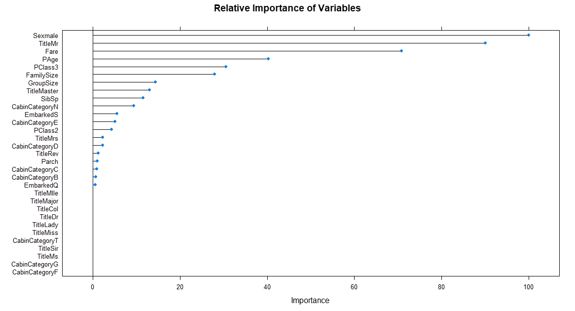
According to the above performance graph, it is clear that “xgbDART” algorithm is showing the highest performance in the 95% confidence level among all models. So, we have selected “xgbDART” as our final algorithm. Let’s see the relative importance of variables used by the final algorithm:
7. Validating Model Performance
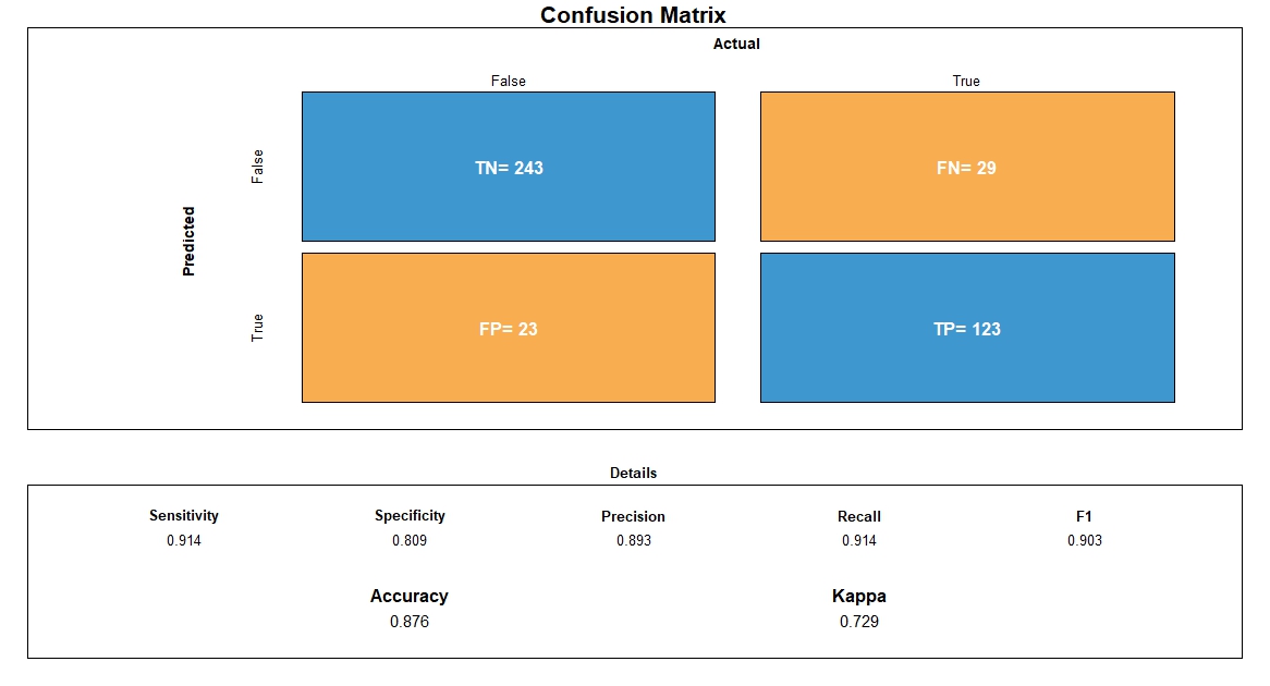
It’s time to validate validation datasets with model of our selected Machine Learning algorithm. After fitting the validation datasets, we got the following confusion matrix. Specificity of the model is 80.9% and sensitivity of the model is 91.4%. Overall performance of the model is 87.6%. So, the accuracy level of the model is very good. Now, let’s see the different parameter values of confusion matrix below:
Conclusion
Hope you have enjoyed the write-up. For the write-up we have used sample titanic datasets from kaggle. We have used here the most popular open source Data Analytics software R and different R supported Machine Learning algorithms to solve the business problem. If you have any query related to this write-up, please feel free to write your comments on our facebook page. Please note that the purpose of this write-up is not to introduce the script of R but is to make you understand the step by step process of Data Analytics as well as application of Machine Learning in the real business world. Next time we will come with another example of another type of solution. If you want to get updated, you can subscribe our facebook page http://www.facebook.com/LearningBigDataAnalytics.

Breast Cancer Prediction Using Machine Learning

Using Cursors to Update Records in SQL Server
How to Get Current Date Without Time in SQL Server
About The Author
Minhajur Rahman Khan
Professional Experience in Machine Learning with R & Python, Oracle Certified Associate, Google Certified Data Analytics Specialization, IBM Certified Data Science Professional, IBM Certified Data Analyst Professional... For more details visit: https://www.linkedin.com/in/minhajrk/
Add a Comment
You must be logged in to post a comment.
Comment