Bank Loan Creditability Prediction Using Machine Learning
As lending is the primary business of the banks, banks have to always find the right customer to lend at low risk to avoid any future non-performing loans. If a bank approves a loan to a borrower and if borrower not repaying the principal amount, bank will lose the principal and interest income. Thus credit risk assessment is very critical while approving a loan to customer.
For most banks, loans are the largest and most obvious source of credit risk, however, other sources of credit risk exist throughout the activities of a bank, including in the banking book and in the trading book, and both on and off the balance sheet. Banks are increasingly facing credit risk in various financial instruments, loan is one of them. Since exposure to credit risk continues to be the leading source of problems in banks world-wide, banks and their supervisors should be able to draw useful lessons from past experiences.
Presently we see that different multinational banks as well some local bank introduced Data Analytics department to utilize data mining techniques which helps them compete in the market and provide the right product to the right customer with less risk. Credit risks which account for the risk of loss and loan defaults are the major source of risk encountered by banking industry. Data mining techniques like classification and prediction can be applied to overcome this to a great extent.
In this article we will show you a step by step process of loan creditability prediction using Machine Learning.
1. Understanding The Datasets
Before starting work we have to have a clear idea about the dataset. Now, let’s see the dataset from different angles.
‘data.frame’: 1000 obs. of 21 variables:
$ creditability : int 1 1 1 1 1 1 1 1 1 1 …
$ account_balance : int 1 1 2 1 1 1 1 1 4 2 …
$ duration_of_credit_in_month : int 18 9 12 12 12 10 8 6 18 24 …
$ payment_status_of_previous_credit : int 4 4 2 4 4 4 4 4 4 2 …
$ purpose_of_credit : int 2 0 9 0 0 0 0 0 3 3 …
$ credit_amount : int 1049 2799 841 2122 2171 2241 3398 1361 1098 3758 …
$ value_savings_stocks : int 1 1 2 1 1 1 1 1 1 3 …
$ length_of_current_employment_in_years: int 2 3 4 3 3 2 4 2 1 1 …
$ installment_percent : int 4 2 2 3 4 1 1 2 4 1 …
$ sex_marital_status : int 2 3 2 3 3 3 3 3 2 2 …
$ guarantors : int 1 1 1 1 1 1 1 1 1 1 …
$ duration_in_current_address_in_years : int 4 2 4 2 4 3 4 4 4 4 …
$ most_valuable_available_asset : int 2 1 1 1 2 1 1 1 3 4 …
$ age_in_years : int 21 36 23 39 38 48 39 40 65 23 …
$ concurrent_credits : int 3 3 3 3 1 3 3 3 3 3 …
$ type_of_apartment : int 1 1 1 1 2 1 2 2 2 1 …
$ no_of_credits_at_this_bank : int 1 2 1 2 2 2 2 1 2 1 …
$ occupation_category : int 3 3 2 2 2 2 2 2 1 1 …
$ no_of_dependents : int 1 2 1 2 1 2 1 2 1 1 …
$ has_telephone : int 1 1 1 1 1 1 1 1 1 1 …
$ is_foreign_worker : int 1 1 1 2 2 2 2 2 1 1 …
Let’s see the meaning of the different fields of the titanic dataset:
creditability : 1 : credit-worthy, 0 : not credit-worthy
account_balance : 1 : no running account, 2 : no balance or debit, 3 : 0 <= … < 200 DM, 4 : >= 200 DM or checking account for at least 1 year
duration_of_credit_in_month : Duration in months
payment_status_of_previous_credit : 0 : hesitant payment of previous credits, 1 : problematic running account / there are further credits running but at other banks, 2 : no previous credits / paid back all previous credits, 3 : no problems with current credits at this bank, 4 : paid back previous credits at this bank
purpose_of_credit: 0 : other, 1 : new car, 2 : used car, 3 : items of furniture, 4 : radio / television, 5 : household appliances, 6 : repair, 7 : education, 8 : vacation, 9 : retraining, 10 : business
credit_amount : Amount of credit in DM
value_savings_stocks : Value savings or stocks. 1 : not available / no savings, 2 : < 100,- DM, 3 : 100,- <= … < 500,- DM, 4 : 500,- <= … < 1000,- DM, 5 : >= 1000,- DM
length_of_current_employment_in_years : Applicant employed by current employer in years. 1 : unemployed, 2 : <= 1 year, 3: 1 <= … < 4 years, 4: 4 <= … < 7 years, 5 : >= 7 years
installment_percent : Installment in percentage of available income. 1 : >= 35%, 2: 25% <= … < 35%, 3: 20 <= … < 25%, 4: < 20%
sex_marital_status : 1 : male: divorced / living apart, 2 : male: single, 3 : male: married / widowed, 4 : female:
guarantors : 1 : none, 2 : Co-Applicant, 3: Guarantor
duration_in_current_address_in_years : 1 : < 1 year, 2 : 1 <= … < 4 years,3 : 4 <= … < 7 years, 4 : >= 7 years
most_valuable_available_asset : 1 : not available / no assets, 2 : Car / Other, 3 : Savings contract with a building society / Life insurance, 4 : Ownership of house or land
age_in_years : Applicant age in years
concurrent_credits : 1 : at other banks, 2 : at department store or mail order house, 3 : no further running credits
type_of_apartment : 1 : free apartment, 2 : rented flat, 3: owner-occupied flat
no_of_credits_at_this_bank : Number of previous credits at this bank (including the running one). 1 : one, 2 : two or three, 3 : four or five, 4 : six or more
occupation_category : 1 : unemployed / unskilled with no permanent residence, 2 : unskilled with permanent residence, 3 : skilled worker / skilled employee / minor civil servant, 4 : executive / self-employed / higher civil servant
no_of_dependents : Number of persons entitled to maintenance. 1 : 3 and more, 2: less than 3
has_telephone : 1 : No, 2 : Yes
is_foreign_worker : 1 : Yes, 2 : No
Let’s see the dataset in more details way with one of my own developed functions:
| variable_name | variable_type | record_count | unique_count | empty_count | null_count | missing_count | |
| 1 | creditability | numeric | 1000 | 2 | 0 | 0 | 0 |
| 2 | account_balance | numeric | 1000 | 4 | 0 | 0 | 0 |
| 3 | duration_of_credit_in_month | numeric | 1000 | 33 | 0 | 0 | 0 |
| 4 | payment_status_of_previous_credit | numeric | 1000 | 5 | 0 | 0 | 0 |
| 5 | purpose_of_credit | numeric | 1000 | 10 | 0 | 0 | 0 |
| 6 | credit_amount | numeric | 1000 | 923 | 0 | 0 | 0 |
| 7 | value_savings_stocks | numeric | 1000 | 5 | 0 | 0 | 0 |
| 8 | length_of_current_employment_in_years | numeric | 1000 | 5 | 0 | 0 | 0 |
| 9 | installment_percent | numeric | 1000 | 4 | 0 | 0 | 0 |
| 10 | sex_marital_status | numeric | 1000 | 4 | 0 | 0 | 0 |
| 11 | guarantors | numeric | 1000 | 3 | 0 | 0 | 0 |
| 12 | duration_in_current_address_in_years | numeric | 1000 | 4 | 0 | 0 | 0 |
| 13 | most_valuable_available_asset | numeric | 1000 | 4 | 0 | 0 | 0 |
| 14 | age_in_years | numeric | 1000 | 53 | 0 | 0 | 0 |
| 15 | concurrent_credits | numeric | 1000 | 3 | 0 | 0 | 0 |
| 16 | type_of_apartment | numeric | 1000 | 3 | 0 | 0 | 0 |
| 17 | no_of_credits_at_this_bank | numeric | 1000 | 4 | 0 | 0 | 0 |
| 18 | occupation_category | numeric | 1000 | 4 | 0 | 0 | 0 |
| 19 | no_of_dependents | numeric | 1000 | 2 | 0 | 0 | 0 |
| 20 | has_telephone | numeric | 1000 | 2 | 0 | 0 | 0 |
| 21 | is_foreign_worker | numeric | 1000 | 2 | 0 | 0 | 0 |
In the above data we see that there is no missing values in the dataset. Actually dataset is fully ready to work with.
2. Visualize The Datasets
Let’s visualize the dataset to understand the business from birds eye.
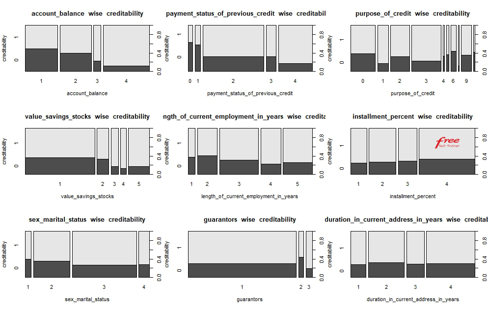
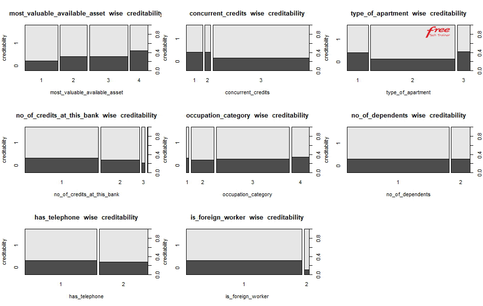
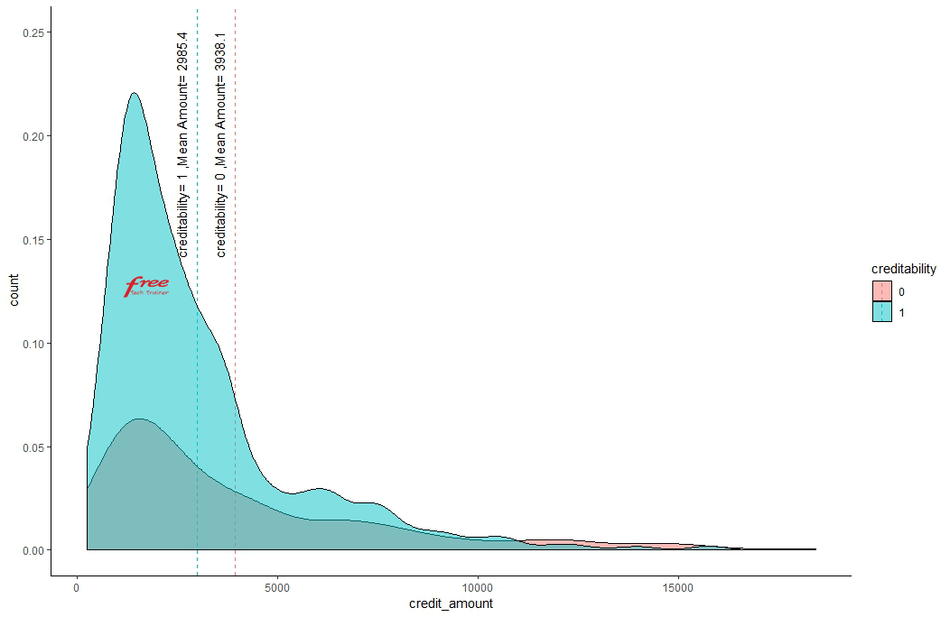
Higher the credit amount higher the risk of creditability.
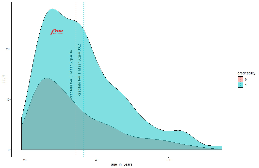
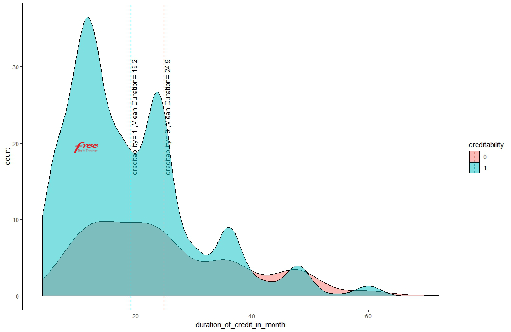
Higher the duration of credit amount, higher the risk of creditability.
3. Importance Features Selection
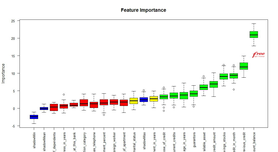
There are 20 independent features in the dataset. Should we consider all of the variables? No, we should not use all of the variables if some of them are not important. To find out important features we can follow manual feature selection process or we can use different algorithms to find them. I would recommend you to use algorithm for this purpose. Here is the recommended features with features importance with the help of one of the algorithms.
4. Training Models
Now we are ready to train our machine using different machine learning algorithms. There are many algorithms in R to train our machine. We have used 15 most popular algorithms to train our machine using training dataset and have built 15 different models. Overall process will take a good amount of time to train our machine with those selected algorithms. It will depends mainly on the capacity of processor & random access memory of our machine.
5. Selecting The Best Model
After completion of the model building process, we have to see the performance of different models. One algorithm can not be the best for all kinds of datasets. It’s time to measure the performance of different models. Let’s see the performance of these 15 models using 15 Machine Learning algorithms:
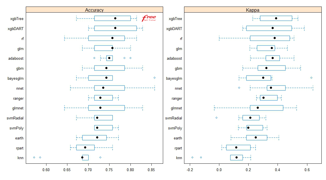
According to the above performance graph, it is clear that “xgbTree” algorithm is showing the highest performance in the 95% confidence level among all models. So, we have selected “xgbTree” as our final algorithm. Let’s see the relative importance of variables used by the final algorithm:
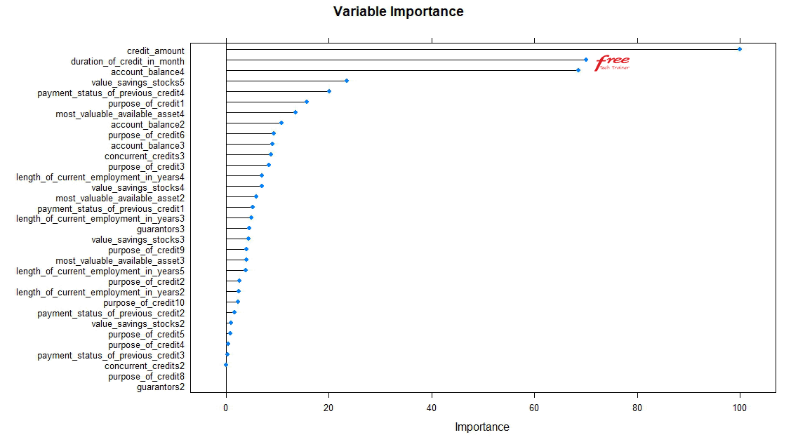
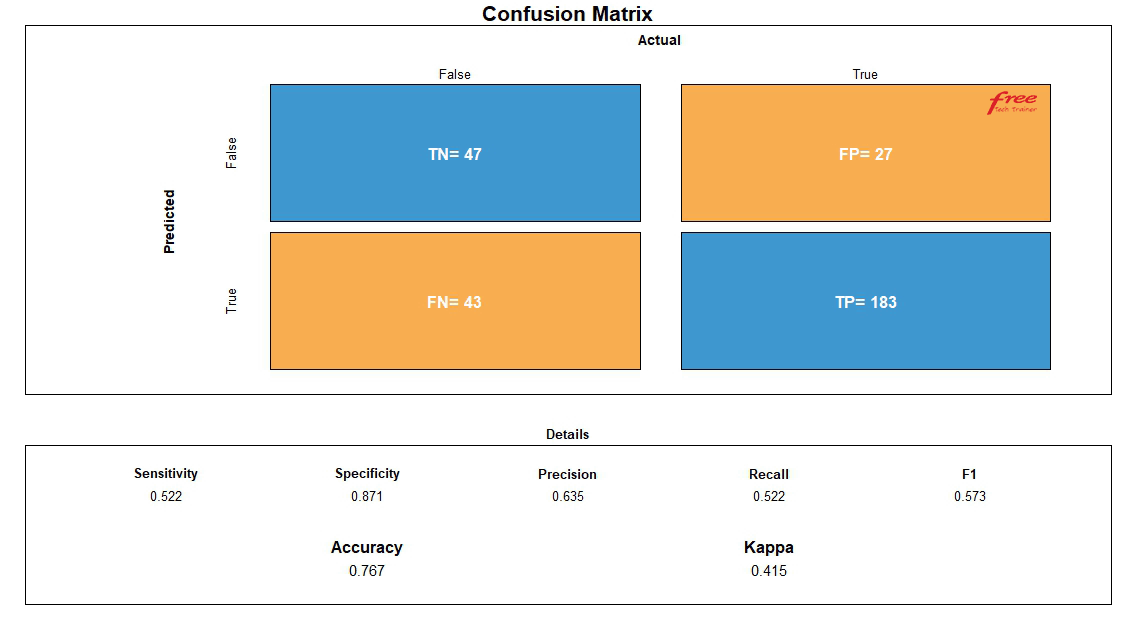
It’s time to test with the test datasets with model of our selected Machine Learning algorithm. After fitting the test datasets, we got the following confusion matrix. Specificity of the model is 87.1% and sensitivity of the model is 52.2%. Overall performance of the model is 76.7%. So, the accuracy level of the model is good. Now, let’s see the different parameter values of confusion matrix below:
Conclusion
Hope you have enjoyed the write-up. For the write-up we have used sample German Credit datasets from web. We have used here the most popular open source Data Analytics software R and different R supported Machine Learning algorithms to solve the business problem. If you have any query related to this write-up, please feel free to write your comments on our facebook page. Please note that the purpose of this write-up is not to introduce the script of R but is to make you understand the step by step process of Data Analytics as well as application of Machine Learning in the real business world. Next time we will come with another example of another type of solution. If you want to get updated, you can subscribe our facebook page http://www.facebook.com/LearningBigDataAnalytics.

